Kalman Filter

Pendulum Dynamics

We will explore the use of a Kalman Filter to estimate the state of a free pendulum starting from an initial state with damped oscillation. We will first explore the use of a linear Kalman Filter based on a linearized model of the pendulum dynamics. Then, we will look at using an Extended Kalman Filter to estimate the states.

The following are the dynamics of the system:

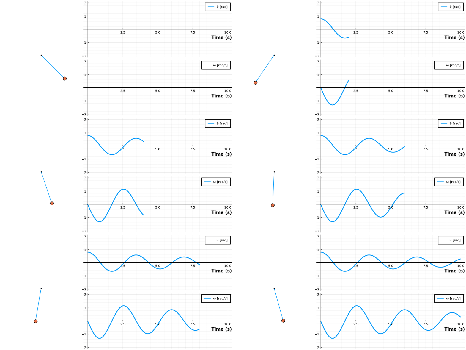
Let's integrate this over a fixed time interval with an initial state.

using Plots
using DifferentialEquations

# Pendulum Parameters
m = 0.5;  # Mass of the pendulum
b = 0.25; # Damping Coefficient
L = 2.8;  # Length of the Pendulum 
g = 9.81; # Gravitational Constant, the average nominal value on Earth,
          # not necessarily where you are standing right now. In fact, the gravitational constant varies 0.7% 
          # across different earth locations, but let's get back to our lesson. 

function pendulum!(dx, x, p, t)
    dx[1] = x[2]; 
    dx[2] = -b/(m*L)*x[2] - g/L * sin(x[1])
end

θₒ = π/4;
ωₒ = 0;
xₒ = [θₒ, ωₒ];

Δt = 0.1; 

tspan = (0.0, 10.0)

prob = ODEProblem(pendulum!,xₒ,tspan)
sol = solve(prob, saveat = Δt)
t = sol.t

function draw_pendulum(θ_list)
    L = 1;
    local p = plot()
    for θ in θ_list
        plot!(p, [0,L*sin(θ)], [0,-L*cos(θ)],size=(300,300),xlim=(-1.2*L,1.2*L),ylim=(-L*1.2,1),ms=2, markershape = :hexagon,label ="", axis = []);
        plot!(p, [L*sin.(θ)], [-L*cos.(θ)], ms=8, markershape = :circle, label ="", aspect_ratio = :equal, showaxis = false);
    end
    return p
end

anim = @animate for i ∈ 1:length(t)
    panim = draw_pendulum([sol[1,i]])
    local p = plot(sol[1:i], lw=2, label=["θ [rad]" "ω [rad/s]"], layout=(2,1))
    plot(panim, p, layout=grid(1, 2, widths=[0.35 , .65]), size=size=(800, 400))
end

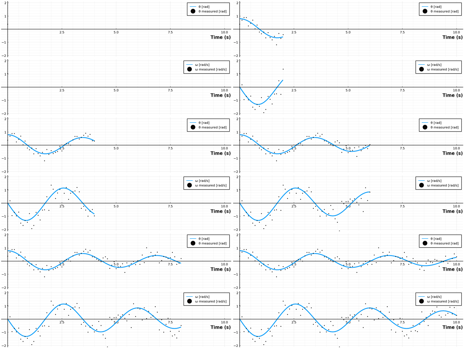
Now let us assume we want to measure the angular position and angular velocity, but we don't have a sophisticated measurement device and so the measurements are noisy. Let's assume the measurement noise is white, Gaussian, not correlated and with zero-mean. Let's add that affect onto the process. Assume the measurements are taken at a sample time of $\Delta t = 0.1 s$

using LinearAlgebra
σ_θ = .25;
σ_ω = .5;
rms(x) = norm(x)/sqrt(length(x))
noise = [σ_θ*randn(length(t))'; σ_ω*randn(length(t))'] 
sol_noisy = zeros(size(sol))
sol_noisy = sol + noise
ϵ = (sol-sol_noisy)
@show ϵ_rms = [rms(ϵ[1,:]),  rms(ϵ[2,:])]


anim = @animate for i ∈ 1:length(t)
    local p = plot(sol[1:i], lw=2, label=["θ [rad]" "ω [rad/s]"], layout=(2,1))
    scatter!(p, t[1:i], sol_noisy[:,1:i]', label=["θ measured [rad]" "ω measured [rad/s]"], ms=1, layout=(2,1))
end

ϵ_rms = [rms(ϵ[1, :]), rms(ϵ[2, :])] = [0.24841861668835655, 0.5037134425875269]

Now this may be an exaggerated noise level, we can change the standard deviation of the measurement noise to make it better or worst, but let's keep it and see how well a Kalman Filter can perform.

Linear Kalman Filter

We clearly don't have a decent measurement system, let's try to apply a Kalman Filter to better estimate our states. Here is a summary of the Kalman Filter for a Continuous-Discrete Time-Invariant Linear System.

The continuous part is the model or process (the pendulum is a continuous system) and the discrete part is the measurement (we take readings at discrete intervals).

Given the dynamic system:

Initialized as follows:

$\hat{x}(0)=E(x_0)=\bar{x}_0\\$ $P(0)= E[(x_0 -\hat{x}(0))(x_0 -\hat{x}(0))^T]=P_0\\$

The time-update (process-update) is in the continuous domain

Numerically integrate with $\Delta t$ as the time step

$\hat{x}^-=\hat{x} + \dot{\hat{x}} \Delta t\\\\$ $P^- = P + \dot{P}\Delta t\\$

And then a measurement-update in discrete form

$K =P^- H^T {(H P^- H^T +R )}^{-1}\\\\$ ${\hat{x} } ={\hat{x} }^- +K (y -H {\hat{x} }^- )\\\\$ $P=(I-K H )P^- {(I-K H )}^T +K R K^T=(I-K H )P^-\\$

Here $\hat{x}^+$, the aposteriori estimate, is expressed as $\hat{x}$

We have to linearize our pendulum system before we use the Kalman Filter above, let's assume a small angle approximation, this would result in the system:

@show A = [0 1; -g/L -b/(m*L)]
B = [0; 0]; H = [1 0; 0 1];

n = 2; # Number of States
m = 2; # Number of Outputs
points = length(t); # Number of measurements 

@show Q = [0.1^2 0; 0 0.25^2];
@show R = [σ_θ^2 0; 0 σ_ω^2]

P = zeros(n, n, points);
K = zeros(n, m, points);

P[:,:,1] = diagm([0.01^2, 0.01^2]);

x̂ = zeros(n, points);
x̂[:,1] = xₒ;
z = sol_noisy;

for k in 2:length(t)
    # Time update a.k.a Prediction a.k.a State Propagation
    ẋ = A * x̂[:,k-1];
    Ṗ = A * P[:,:,k-1] + P[:,:,k-1] * A' + Q; 

    # Integrate to propagate apriori state and apriori covariance
    x̂⁻ = x̂[:,k-1] +  ẋ * Δt
    P⁻ = P[:,:,k-1] + Ṗ * Δt

    # Kalman Gain. Larger gains puts a heavier weight on the measurement and vice versa.
    K[:,:,k] = P⁻*H' * inv( H*P⁻*H' + R);
    
    # Measurements Update 
    x̂[:,k] = x̂⁻ + K[:,:,k] *(z[:,k] - H * x̂⁻);  # aposteriori state estimate update
    P[:,:,k] = (I - K[:,:,k] * H) * P⁻;         # aposteriori error covariance update
end

kf_e = (sol - x̂);
kf_e_rms = [rms(kf_e[1,:]),  rms(kf_e[2,:])]
@show kf_e_rms

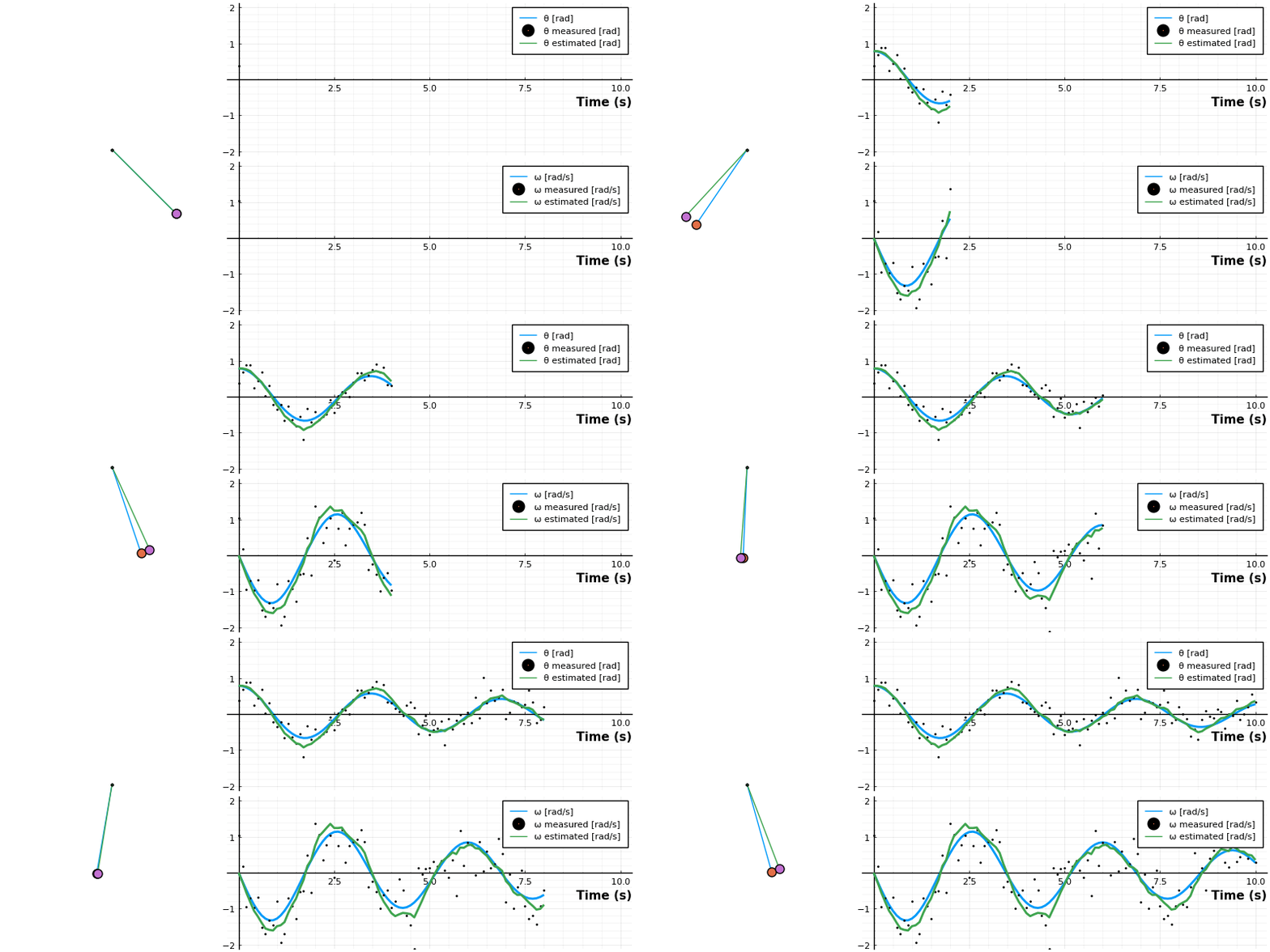
anim = @animate for i ∈ 1:length(t)
    panim = draw_pendulum([sol[1,i] x̂[1,i]])
    local p = plot(sol[1:i], lw=2, label=["θ [rad]" "ω [rad/s]"], layout=(2,1))
    scatter!(p, t[1:i], sol_noisy[:,1:i]', label=["θ measured [rad]" "ω measured [rad/s]"], ms=1, layout=(2,1))
    plot!(p, t[1:i], x̂[:,1:i]', label=["θ estimated [rad]" "ω estimated [rad/s]"], lw=2, layout=(2,1))
    plot(panim, p, layout=grid(1, 2, widths=[0.35 , .65]), size=size=(800, 400))
end

A = [0 1; -g / L -b / (m * L)] = [0.0 1.0; -3.503571428571429 -0.044642857142857144]
Q = [0.1 ^ 2 0; 0 0.25 ^ 2] = [0.010000000000000002 0.0; 0.0 0.0625]
R = [σ_θ ^ 2 0; 0 σ_ω ^ 2] = [0.0625 0.0; 0.0 0.25]
kf_e_rms = [0.08465364260080768, 0.16970747738721473]

What's happening above is that state is propagated by using our knowledge of the pendulum physics (the model), which results in the apriori estimate $\hat{x}^-$.

The covariance matrix $P$ is also propagated through time using the model physics (the $A$ matrix), the covariance matrix holds the stochastic information of each state and the statistical relationship of the states.

Notice that in the situation above, it is independent of the state. In fact, it can be precalculated off-line, and it can converge after a time-period.

# Time update a.k.a Prediction a.k.a State Propagation
ẋ = A * x̂[:,k-1];
Ṗ = A * P[:,:,k-1] + P[:,:,k-1] * A' + Q; 

x⁻ = x̂[:,k-1] +  ẋ * Δt
P⁻ = P[:,:,k-1] + Ṗ * Δt

The time-update step can be done multiple times before the measurement update occurs. You can do 5 process updates for every measurement update for example. Measurement updates can be synchronous or asynchronous as well.

When a new measurement is ready, we perform the measurement update step. We compute the Kalman gain which is a function of the covariance matrix, the sensor (output matrix $H$) and the $R$ matrix which holds the stochastic specification of the measurement model.

# Kalman Gain. Larger gains puts a heavier weight on the measurement and vice versa.
K[:,:,k] = P⁻*H' * inv( H*P⁻*H' + R);

Think of the Kalman Gain as a weighting factor for the measurement versus the process (the estimate from the physics: the integration of the model). If, stochastically, we trust the process more than the measurement, the gain would be low. If we trust the measurement more, then the gain would be high.

Then we use the gain to compute the estimate of the state, called the aposteriori based on the steps above it. As well as update the aposteriori of the covariance matrix

# Measurements Update 
x̂[:,k] = x̂⁻ + K[:,:,k] *(z[:,k] - H * x̂⁻);  # aposteriori state estimate update
P[:,:,k] = (I - K[:,:,k] * H) * P⁻;         # aposteriori error covariance update